HOW TO NOT RUIN YOUR SPREADSHEET
If you have purchased a spreadsheet from us, or if you are using a spreadsheet which has already been made, there are some ways that you can ruin the spreadsheet. We lock our spreadsheets to avoid the formulas from being over-written but, even so, there are ways that you can still ruin the spreadsheets. We always advise that people keep a blank copy of the spreadsheet in a safe folder somewhere. Then if the version that you are using is corrupted, you can always copy your data over to a new clean version. Even if you do that, you still want to avoid unnecessary issues, here are 5 things to avoid when using spreadsheet templates to ensure that you don’t ruin them.
Watch the video or take a look below for written instructions.
WHAT NOT TO DO, AND WHAT TO DO INSTEAD
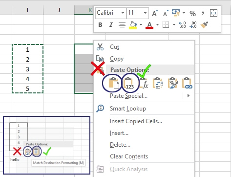
COPY & PASTE – You will probably need to copy and paste data at some point, either internally (from your spreadsheet to another place in your spreadsheet) or externally (from an external spreadsheet to your spreadsheet). Either way you don’t want to use the copy and paste function, nor any shortcuts, to achieve this. Why not? Using copy and paste in Excel, will copy and paste EVERY aspect of the copied section. It won’t just paste the text, but the formatting too. This could cause major issues. The worst of all is if you copy from an external spreadsheet, the cells may be formatted as locked (which is the default). They won’t be locked on the source spreadsheet, as the lock function has not been activated (on the source spreadsheet), but it has been in one of our spreadsheets. This means that you may copy and paste into unlocked cells, but once you have pasted they change to locked cells. This means that the cells you need to access will then be locked. It is not only this, but there may be hidden conditional formatting, which will be ruined using copy and paste. So what do you do then? Simple, just use paste VALUES instead. If you right click and copy, and right click again, you should see the menu shown on the image to the right. If you’re pasting data from an external source, sometimes it doesn’t give you the paste VALUES option, then just select to keep destination formatting.
DRAG – As you may know, you can select the bottom right of a cell, or selection of cells, and drag it down in order to extend the selection. We don’t blame you for using this, as it is extremely useful, however it is the same as copying and pasting. This means that it will do the same as the first point. How do you overcome this? Don’t use that function, use the copy and paste VALUES as above.
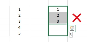
DELETING DATA – When you’re making your own spreadsheet, and you delete data, you will notice that it removes the cells and moves the rest up. I’m sure you can imagine that this will be disastrous for any formulas which aren’t visible to you. Now usually if the spreadsheet is locked, you won’t be able to delete cells, but this is a good practice to do anyway. If you want to remove data in some cells, but don’t want to ruin the integrity of the spreadsheet, simply use CLEAR CONTENTS instead. When you’re using a pre-made spreadsheet, this will remove the unwanted data, but keep the spreadsheet in tact. If you remove unwanted data, and the data left is not neat and tidy, then use the sort function (if available) to sort the data.
MOVING DATA – Don’t grab cells and move them to another location. This messes up all the formulas referencing those cells and will leave you with #REF errors and a broken spreadsheet. To ‘move’ data simply copy the data, paste (using paste VALUES) where you want the data, and then clear the old data using clear contents.

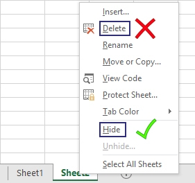
HIDING SHEETS – We are able to lock spreadsheets (sheets) without locking the workbook. This means that individual sheets may be locked, but you can rename tabs, or delete sheets. Sometimes we need to leave this function unlocked, in order for you to hide certain tabs during certain times. In this case, you will be able to hide (or unhide) tabs by right clicking on the selected tab (or any other when it comes to using the unhide function). Make sure you DO NOT use the Delete option. This will delete the tab, and you can’t get it back. Even clicking the back arrow won’t get it back. So if you do want to hide a tab, make sure you hide it and don’t delete it.
HOW TO RESTORE YOUR SPREADSHEET
If you’re using Office 365, you can always restore an older version if you have corrupted a spreadsheet. If you need to use a new spreadsheet (if you’ve ruined the old one, or had upgrades done and now have a new blank spreadsheet), then the best thing to do is transfer the data from the old spreadsheet to the new one. It will not transfer errors that have been created by making the mistakes mentioned above, as long as you follow these rules:
- Always use copy and paste VALUES never normal paste (or any others).
- Copy and paste (VALUES) each set of unlocked cells at a time, don’t include any locked cells in your selection.
- Make sure that you ‘transfer’ ALL data and that it is pasted (using paste VALUES) in the correct locations (under the right column headers and in the right rows).
If you use this method, you copy the data from the corrupted or incorrect spreadsheet, and then paste values (only the data, not the issues) into a new spreadsheet. The new spreadsheet will then do what it has been designed to do using the inputted data.
We hope that this helps you, if you’re still stuck and you’re using one of our spreadsheets, please get in touch.
COPYING AND PASTING BATCHES OF DATA
If you need to copy and paste batches of data from one spreadsheet to another, from an existing spreadsheet into another location in the same spreadsheet, or from an older version to a newer version, here is a video to help.
This is a video from my Excel Help range of videos.